Storage Engines from first principles
Published
Your bar: redraw — from memory — how a database puts bytes on disk and finds them again, so you can choose engines, indexes, and data models with judgment instead of cargo-culting. Every level is built to be seen and redrawn. Grounded in Kleppmann’s Designing Data-Intensive Applications 1 and the primary papers behind each engine.
One tension holds the whole book. Each level just moves you along its curve:
A storage engine is a log you write
plus an index you read
trading read / write / space
to fit one access pattern
Log + hash index — the simplest real engine
Two lines of bash become a durable database — and reveal the tension that governs every index you’ll ever choose.
key → offset in RAM. Reads do one
lookup + one seek regardless of file size.6 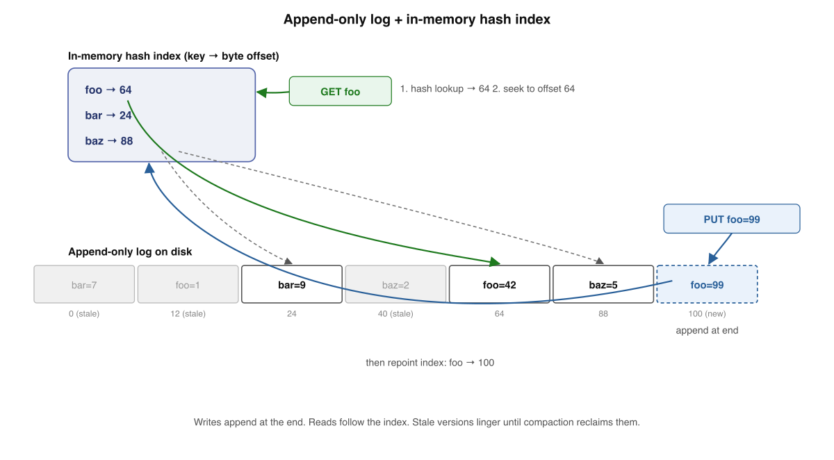
The same idea from the book: writes stream to the tail; the hash map turns “search the data” into “consult a small structure, then seek.”
Is An append-only log of key,value records + an in-RAM map from each
key to its latest byte offset.
Why it exists Appends are the fastest write a disk offers — one position, then stream. The index converts a scan into a seek.
Compaction Segments close at a size cap, become immutable, and a background merge keeps only the latest value per key.
Like (code) A SELECT … LIMIT 1 over a tail-appended file, but the
offset is precomputed in a hash map.
✓ Compaction rewrites a fresh segment, swaps it atomically, deletes the old — crash-safe by immutability
📜 Memory rule: A storage engine is a log you write fast and an index you read fast — and every index you add taxes every write.
Memory check
- Why is
db_setfast butdb_getslow without an index? → append vs full linear scan - What does Bitcask's hash map store? → key → byte offset of latest record
- Why can compaction run without blocking reads? → new segment swapped in atomically; old stays immutable
B-tree — the read-optimized default
The structure behind every CREATE INDEX since 1972: a shallow, sorted,
page-oriented tree you update in place.
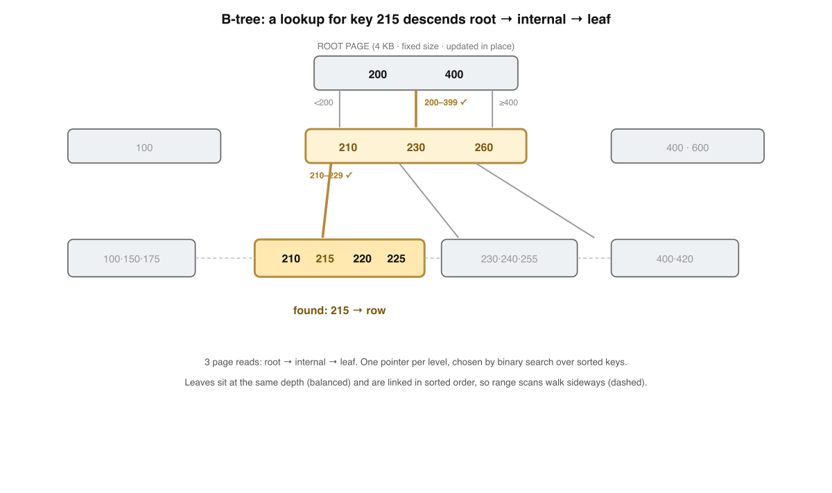
Lookup of key 215: root [200,400] → internal [210,230,260] →
leaf. Three page reads, each a binary search in memory.
Is A balanced tree of fixed-size pages (4–8 KB); each node is sorted keys + child pointers; all leaves at equal depth.
Why it exists A high branching factor keeps the tree shallow, so a point lookup is O(log n) pages — and range scans walk the sorted leaves.
Update-in-place One canonical location per key; a write overwrites the leaf page. A full leaf splits and pushes a separator up.
Crash safety Overwriting a page isn’t atomic, so the WAL records intent first; recovery replays it. 1
✓ Depth grows logarithmically — fan-out ~256 means 4 levels hold ~4 billion keys
🌳 Memory rule: A B-tree is sorted pages updated in place — cheap predictable reads, paid for with random write I/O and WAL.
Memory check
- What keeps a B-tree lookup to a few reads at a billion rows? → high branching factor → shallow tree
- What happens when a leaf has no room? → split in two, push a separator to the parent
- Why does a B-tree need a WAL? → in-place page overwrite isn't crash-atomic
LSM-tree — write-optimized, log all the way down
Turn every write into a sequential append; defer the cleanup to a background merge. The engine behind RocksDB & Cassandra.
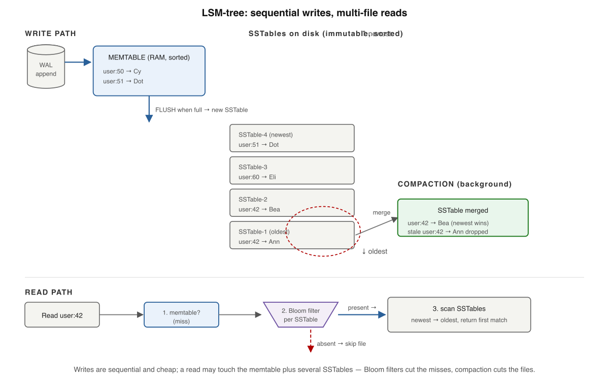
Write → WAL + memtable; flush a full memtable as a new immutable SSTable; compaction merges runs; reads go memtable → SSTables newest-to-oldest, gated by Bloom filters. 3
Memtable In-RAM sorted map (skip list / RB-tree) that buffers writes; a WAL alongside makes it crash-safe.
SSTable Immutable on-disk file sorted by key — never modified, only merged away. Two sorted files merge in one linear pass.
Updates & deletes are writes too An update appends a newer entry; a delete appends a tombstone. Old values are shadowed, not erased.
Compaction Merges runs, keeps the newest value per key, drops tombstoned keys — reclaiming space. Leveled vs size-tiered is a tunable knob.
✓ A tombstone shadows the value; space returns only when compaction reaches the oldest
SSTable (Cassandra: gc_grace_seconds)
🪵 Memory rule: An LSM-tree buffers in RAM, flushes immutable sorted runs, and merges later — sequential writes now, read & merge work deferred.
Memory check
- Why are LSM writes fast? → append to WAL + insert into in-RAM memtable; no in-place disk write
- A read returns "not found" but old SSTables have a value — why? → a newer tombstone shadows them
- What guarantee does a Bloom filter give? → "definitely absent" is never wrong → safe to skip
Amplification — the three currencies you trade
Read, write, space: a logical op costing more than one physical op. You can’t drive all three to zero — pick a corner.
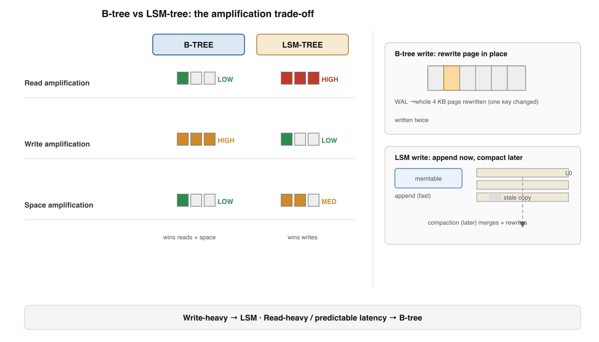
The amplification grid from the book: where each engine spends, where each saves. B-tree pays write; LSM pays read & space-until-compacted. 1
| Axis | B-tree | LSM-tree |
|---|---|---|
| Read amp | low — bounded by tree height | medium–high — may probe many runs |
| Write amp | medium–high — in-place, random, WAL + page | low now — deferred into compaction |
| Space amp | low — one copy, page slack | medium — stale versions until compacted |
| Write I/O | random | sequential |
| Latency | predictable | spiky (compaction stalls) |
Read amp Pages touched per logical read. B-tree ≈ 1 uncached (the leaf); LSM grows with the number of sorted runs.
Write amp Bytes written per byte of user data. B-tree: WAL + whole-page rewrite + splits. LSM: defers & batches into big sequential rewrites.
Space amp Disk used vs logical data. B-tree: page slack (~60–70% full). LSM: stale versions + tombstones, often offset by compression.
Choose by workload Write-heavy ingest → LSM. Read-heavy, tail-latency-sensitive OLTP → B-tree.
✓ They defer and batch it into compaction — a key may be rewritten across several levels over its life
⚖️ Memory rule: Read, write, space — every engine picks one corner of the triangle and pays in the other two. The skill is reading the workload.
Memory check
- Why is an LSM point lookup sometimes slower than a B-tree's? → key may live in any of several sorted runs
- Why does a tiny B-tree update still amplify writes? → rewrites a whole page + a WAL record
- Where does LSM space amp come from? → stale versions + tombstones held until compaction
Indexes — clustered vs secondary, and the write tax
One set of rows, many access paths. Every secondary index is pure redundancy you build, pay for, and keep in sync.
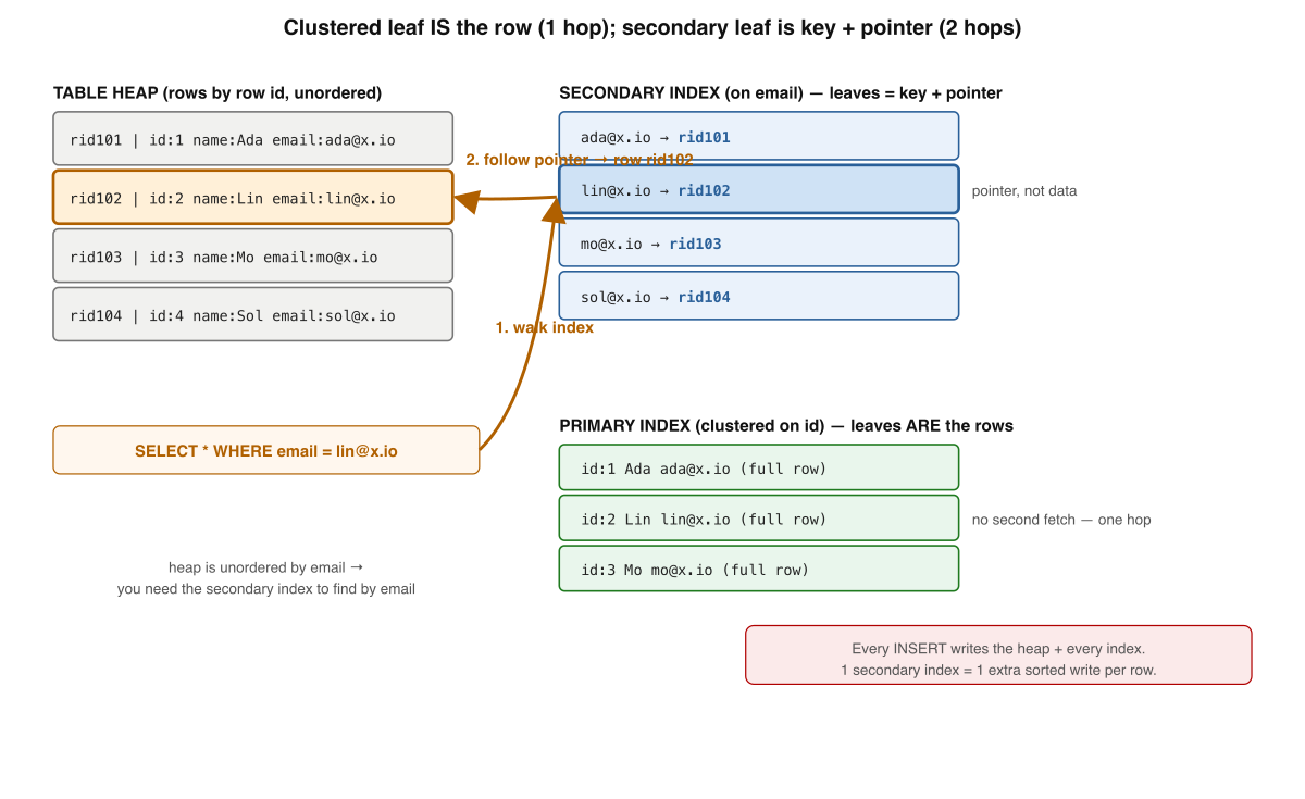
Clustered (InnoDB): the row lives in the PK leaf, secondaries store the PK. Heap
(Postgres): rows in a heap, every index holds a ctid pointer.
Clustered The PK B-tree leaf is the row (InnoDB). A secondary stores the PK value → secondary lookup walks two trees.
Heap Rows sit unordered in a heap; every index leaf holds a ctid
pointer (Postgres). PK lookup = index walk + heap fetch.
Composite Keyed on several columns, sorted lexicographically. Usable only for a left-anchored prefix (leftmost-prefix rule).
Covering Holds every column the query reads, so the answer comes from the index alone — no row fetch.
✓ A table with 8 indexes turns 1 logical insert into 9 physical writes; each index is a standing write tax
🔎 Memory rule: An index makes reads it covers faster and every write that
maintains it slower — index what you actually filter and sort by, and measure with
EXPLAIN.
Memory check
- What does an InnoDB secondary index store in its leaf? → the indexed value + the primary key
- Which query can't use
(account_id, created_at)? → one filtering only on created_at - Why does each secondary index slow writes? → every write must place/move the key in that index too
Data models — relational, document, graph
The most consequential, hardest-to-change backend decision. Each model makes a different relationship cheap.
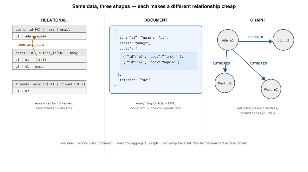
The same user-posts-friends domain modeled three ways: relational tables joined by value, one embedded document, a property graph of traversable edges. 4
Relational Rows relate by value (foreign key); a join assembles them at query time. No duplication, referential integrity, ad-hoc queries.
Document One self-contained JSON/BSON tree embedding related data — great locality, eases the object-relational impedance mismatch.
Graph Nodes + labeled directed edges; an edge is a traversable pointer (index-free adjacency), so a hop is O(local fan-out), not a fresh search.
Convergence Postgres jsonb stores an indexable document in a
relational row — the choice is increasingly per-field.
✓ Each model is a locality bet; relational stays the safe default when access patterns are unknown (Codd separated logical from physical)
🗂️ Memory rule: Pick the model whose cheap operation is what your app reads and traverses most — not the trendiest one.
Memory check
- How does relational relate two rows? → by value — a FK matching another table's PK
- Why is embedding posts in a user doc fast to read? → one contiguous fetch returns the whole aggregate
- Why is a graph good at deep traversals? → each hop follows a stored edge, not a fresh index lookup
Normalization vs denormalization — where each fact lives
Store a fact once and the database protects it. Copy it for speed and you inherit the job of keeping every copy honest.
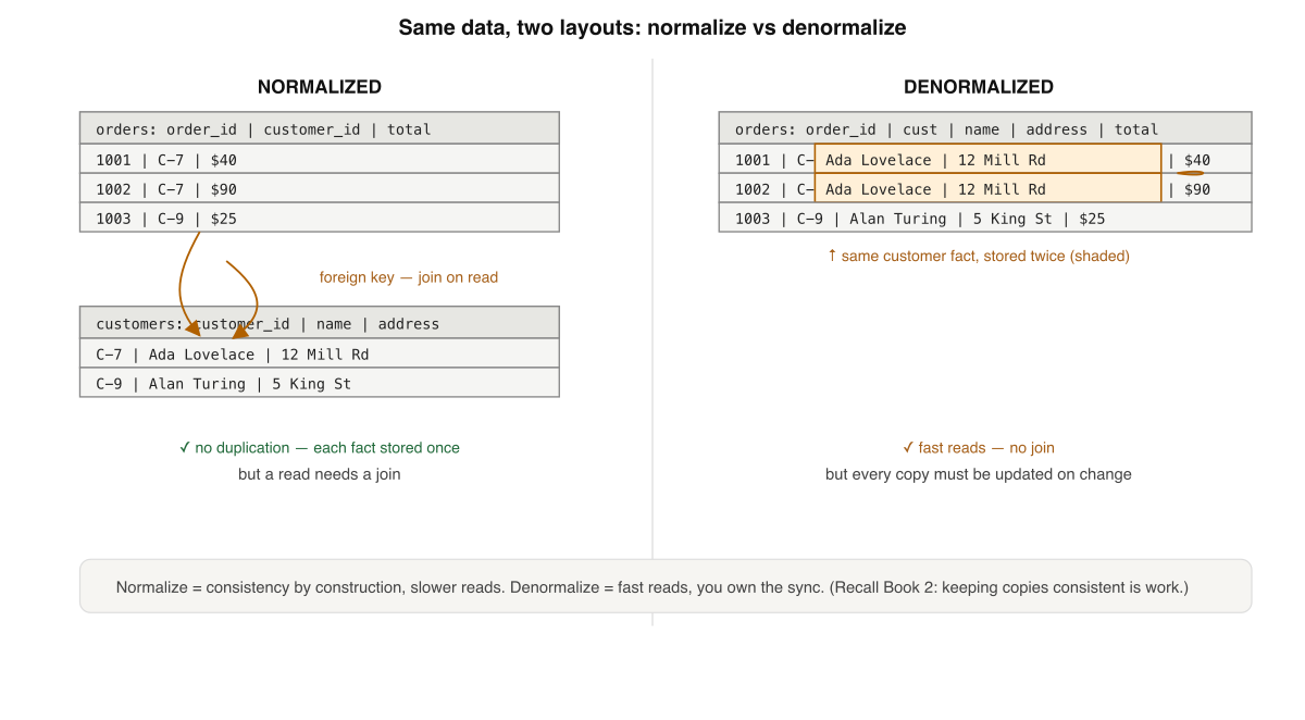
Normalized: customer stored once, joined on read. Denormalized: customer copied into every order — single-row reads, but a change fans out.
| Normalized | Denormalized | |
|---|---|---|
| Each fact | stored once | stored many times |
| Read “order + customer” | join | single row |
| Address change | one update | fan-out update |
| Owns consistency | the database | you (or a materialized view) |
Normalization Each independent fact in exactly one row; everything else references by key. Consistency by construction (1NF→2NF→3NF).
Denormalization Deliberately copy a fact into the rows that read it — join-free reads, paid for with fan-out write sync.
Schema-on-write Relational: columns/types/constraints validated on the way in.
Schema-on-read Document/lake: bytes written as-is, structure interpreted by the reading code — the schema just lives in that code.
✓ The schema still exists — it’s implicit in the reader and can silently drift between versions
📐 Memory rule: Start normalized (correct by construction); denormalize specifically, against a measured read pattern, knowing exactly which invariant you just took ownership of.
Memory check
- What does normalization eliminate? → redundant copies of a fact that drift out of sync
- Copy
customer_nameinto orders — which invariant do you now own? → every copy must update when the customer changes - What decides normalize vs denormalize? → read/write ratio, access pattern, consistency tolerance
Encoding & evolution — bytes that outlive their writer
An in-memory object is a graph of pointers meaningful only in one process. To store or send it, you flatten it — and then change its shape for years without breaking old readers.
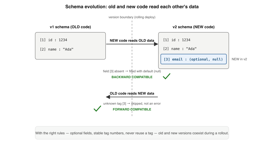
The two crossing arrows: backward (new code reads old data) and forward (old code reads new data) compatibility — what makes rolling deploys safe. 5
| Field names in bytes | Size | Needs schema to read | |
|---|---|---|---|
| JSON / XML | yes, every record | larger | no |
| Protobuf / Thrift | no — tag numbers | smaller | yes |
| Avro | no identifiers at all | smallest | yes (writer + reader) |
Encoding Flatten a pointer-laced object graph into a self-contained byte sequence; decoding rebuilds it in a possibly different process, months later.
Text vs binary JSON ships field names + decimal text (readable, schema-free). Protobuf/Avro ship tagged values (compact, fast, need a schema).
Backward compat Newer code reads older data — new fields are absent, filled by default.
Forward compat Older code reads newer data — it skips the unknown tag and parses the rest. This is why rolling deploys are safe.
✓ The moment one producer omits it, every old consumer breaks — proto3 removed
required for exactly this
🔁 Memory rule: Encoding choices at write time constrain every reader for the data’s lifetime — which far outlives any one service version. Keep both directions compatible.
Memory check
- Why can't you dump raw in-memory bytes to disk? → pointers are addresses valid only in the writer's process
- Why does old code survive a message from new code? → it skips the unknown tagged field
- Which rule silently corrupts reads if broken? → reusing a retired tag number
Row vs column — match the layout to the workload
The capstone. OLTP wants whole rows by key; OLAP scans millions of rows but a handful of columns. The bytes reorganize entirely.
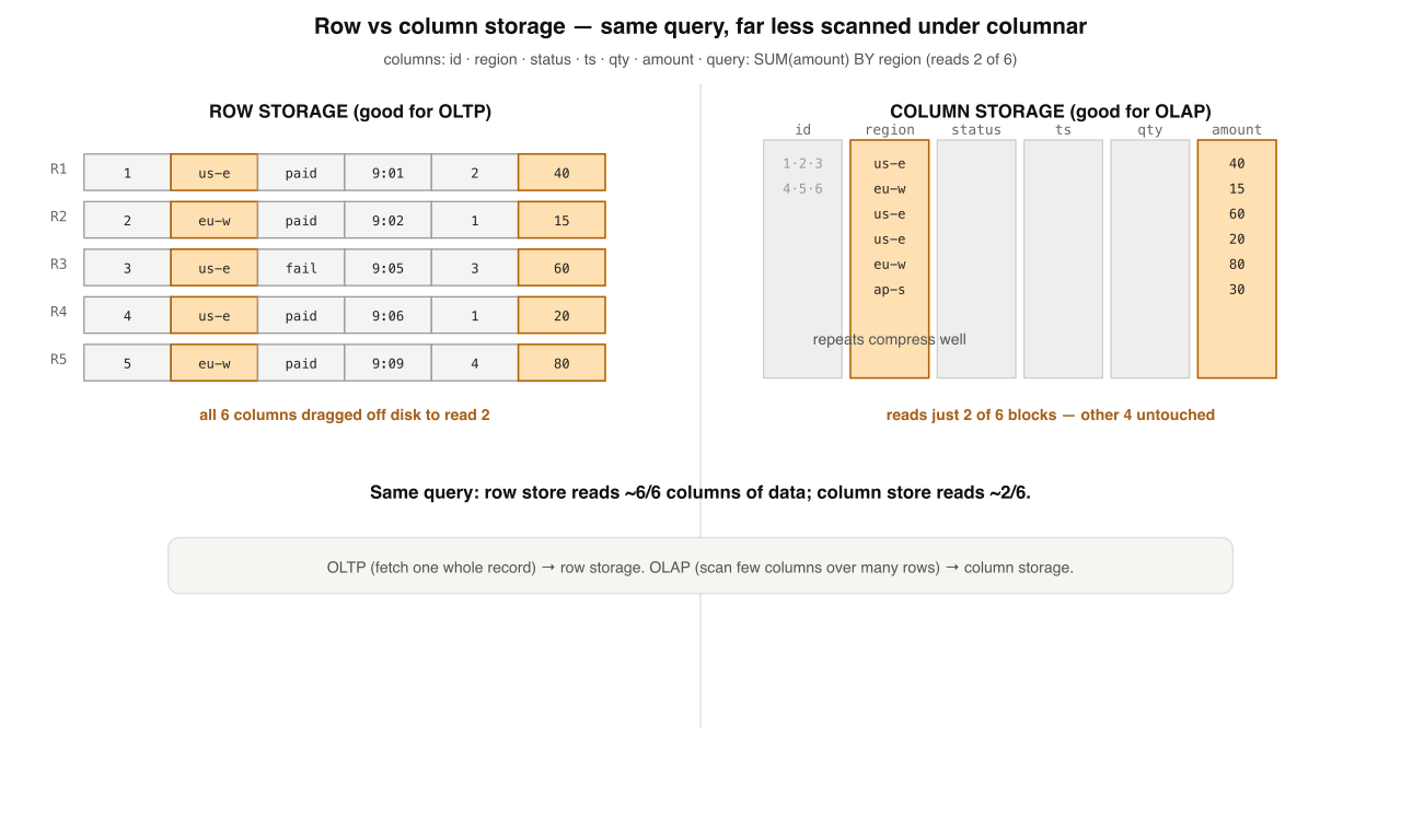
Row store: all of a row’s cells adjacent — perfect for “fetch order #4821”. Column store: all values of one column adjacent — scan reads only the columns named. 7
| OLTP | OLAP | |
|---|---|---|
| Read pattern | few rows, by key | millions of rows, scan |
| Columns touched | all (whole record) | 2–5 of many |
| Write pattern | random inserts/updates | bulk load / append |
| Bottleneck | seek latency | scan bandwidth |
| Layout | row store (B-tree / LSM) | column store (Parquet, Vertica) |
Row store All of a row’s values adjacent. The unit you store together is the unit you retrieve together — ideal OLTP locality.
Column store All values of one column adjacent in its own block; a scan reads only the columns it names, bounded by columns-touched not table-width.
Compression A column is one type from one domain → run-length / dictionary / bitmap encoding compress far harder than a heterogeneous row.
Star schema Warehouses ETL into a column store: a narrow central fact table (one row per event) + small dimension tables radiating out.
✓ Only an engine that fits an access pattern — the same logical table can (and at scale should) live in both a row and a column store
🏛️ Memory rule: Match the storage layout to the workload — many small key reads → row; few wide scans → column. The senior skill is reading the workload, not memorizing engines.
Memory check
- What distinguishes OLAP from OLTP? → scans many rows but reads few columns
- Two reasons columnar scans are fast? → read only needed columns + compress same-domain values
- What does a star-schema fact table hold? → one row per event, FKs out to dimension tables
Where each layer shows up — real engines
Grounding for your judgment: the concept, a concrete engine that embodies it, and the shape the trade-off usually takes.
| Concept | Real engine / feature | The trade-off it makes |
|---|---|---|
| Log + hash index | Bitcask (Riak) | blazing reads, keyset must fit RAM |
| B-tree | PostgreSQL btree · InnoDB clustered PK | low read amp, random write I/O |
| LSM-tree | RocksDB · Cassandra · ScyllaDB | cheap sequential writes, read & compaction cost |
| Amplification knob | RocksDB leveled vs universal compaction | trade write amp against space amp explicitly |
| Clustered vs heap | InnoDB (PK leaf = row) vs Postgres (heap + ctid) | two-tree secondary vs heap pointer chase |
| Document model | MongoDB (16 MB doc cap forces subset pattern) | locality vs unbounded-array bloat |
| Materialized view | Postgres | denormalized read speed vs staleness |
| Encoding / evolution | Protocol Buffers · Avro · Parquet footer | compactness vs human-readability + compat rules |
| Column store | Vertica (C-Store) · Parquet (Dremel) · Citus columnar | fast analytic scans, expensive single-row writes |
Pattern to notice: most “B-tree vs LSM” debates are really amplification debates, and most engines now ship both modes (MyRocks, WiredTiger). Reason about the axes, not the data-structure name. 1
Retrieval practice — mix the levels
Reading builds fluency (feels familiar). Recall builds storage (lasts). Answer from memory — instant feedback.
Q1. What does a Bitcask-style hash index actually map?
Q2. Why does a B-tree need a write-ahead log?
Q3. A read returns "not found", yet older SSTables hold a value. Why?
Q4. Which query can an index on (account_id, created_at) NOT serve efficiently?
Q5. You copy customer_name into every order row. Which invariant do you now own?
Q6. Why does column-oriented storage make analytic scans faster?
Reconstruct the engine from a blank page
Write the nine levels in order, one line each, with nothing on screen. Then reveal and compare — gaps are your next drill.
1 Log + hash index: append data, map key→offset · 2 B-tree: sorted pages, update in place, WAL · 3 LSM: memtable→SSTable→compaction, tombstones, Bloom · 4 Amplification: read/write/space triangle, pick a corner · 5 Indexes: clustered vs heap, composite prefix, covering, write tax · 6 Data models: relational/document/graph by access pattern · 7 Normalize vs denormalize: where each fact lives · 8 Encoding: flatten objects; backward + forward compat · 9 Row vs column: match layout to OLTP vs OLAP.
I’m your teacher — ask me anything. Say “grill me on storage engines”
for mixed no-clue questions, or drop a real workload and I’ll place it on the read↔write
amplification and row↔column axes with you. Want a worked EXPLAIN walkthrough or
the next part (Streaming & Event-Driven)? Just ask.
Interview — pick your bar
Answer out loud in ~60s, then reveal. Core = recall · Senior = trade-offs & failure modes · Staff = synthesis under ambiguity · System Design = open design round (a different axis, not a harder level).
Walk me through what a storage engine does to turn "find me row 42" into disk I/O.
What is a clustered index versus a secondary index, and where does the row actually live?
ctid heap pointer → consequence: a wide PK bloats every secondary index in a clustered engine → a secondary index is pure redundancy you build, pay for on every write, and keep in sync.What is a composite index on (a, b), and which queries can use it?
a then b → so it serves any left-anchored prefix: a=… and a=… AND b=… → it does not serve b=… alone, because there is no left-anchored prefix to seek on → rule of thumb: put the equality column first and the range column second, since a range on the leading column "uses up" the sort order for everything after it → verify with EXPLAIN rather than guessing what the planner picks.What is a write-ahead log (WAL), and why does a B-tree need one?
A teammate says "LSM-trees are just faster than B-trees." Correct them.
Define read, write, and space amplification, and explain why you can't drive all three to zero.
An InnoDB secondary-index lookup is slow. Explain the mechanics and a fix.
EXPLAIN that you actually got the covering/index-only plan.What does the page / buffer cache do, and how does it change how you reason about read cost?
How do you choose between a B-tree (row store) and an LSM-tree for a new service, and how would you defend reversing that choice later?
"Add an index, the query's slow" — make the principal-level case for when not to add one.
EXPLAIN, don't cargo-cult.When is a column store the right call over a row store, and what exactly are you trading?
- Clarify the workload: write:read ratio, point vs range reads, p99 latency target, durability/consistency needs.
- Size it: dataset vs RAM, growth rate, storage budget — does the working set fit the buffer cache?
- Pick the engine corner: B-tree/row for read-heavy OLTP, LSM for write-heavy ingest, column store for analytics scans.
- Index the real predicates: clustered key choice, covering/composite indexes, and the write tax each adds.
- Durability path: WAL/fsync policy, crash recovery, replication.
- Separate OLTP from OLAP: row store + ETL into a columnar warehouse so heavy scans don't starve user I/O.
- Observability & trip-wires: cache hit ratio, p99 read, write/space amp — and the metric that says you chose wrong.
Design the storage for a product with live order pages AND an analytics dashboard.
Design the storage engine + indexing for a write-heavy event-ingest service that also needs fast recent-event reads.
★ Cheat sheet — name → mechanism
Mental models: Log = the fast write · Index = the fast read · B-tree = sorted pages in place · LSM = log + merge · Amplification = the three currencies · Clustered = row in the PK leaf · Heap = row + pointer · Covering = answer from the index alone · Normalize = fact stored once · Denormalize = fact copied · Encoding = flatten the object · Column store = layout for the scan.
Translation table
| Term | What it actually is |
|---|---|
| Storage engine | The layer that lays bytes on disk and finds them again |
| Compaction / VACUUM | Background rewrite reclaiming stale versions & tombstones |
| Write amplification | Bytes physically written per byte of user data |
| Tombstone | An appended delete marker; space returns at compaction |
| Bloom filter | Per-SSTable bit array: “definitely absent” / “probably present” |
| Covering index | Index holding every column the query reads → no row fetch |
| Schema-on-read | Structure interpreted by the reading code, not validated on write |
| Forward compatibility | Old code reads new data by skipping unknown fields |
| Star schema | Narrow fact table + small dimension tables, for column-store OLAP |
Three rules for the architect chair
① There is no best engine — match the layout to the workload (read vs write
vs scan). ② Every index is a read win bought with a write tax; index
deliberately, measure with EXPLAIN. ③ Start normalized;
denormalize against a measured read pattern, knowing which invariant you took on.
★ Review guides & what to read next
5-min (weekly) Don’t re-read — recall. Redraw the amplification triangle; trace a B-tree split and an LSM compaction from memory; recite where each index pays; translate three terms blind.
30-min (when stalled) Blank-page reconstruct all nine levels; re-derive why the log forces an index and the index forces the read/write tension; then place one real workload (which engine? which indexes? row or column?).
Read next, in order: ① DDIA — Kleppmann, ch.3 storage & retrieval (Levels 1–5, 9), then ch.2 data models (6–7) and ch.4 encoding (8) · ② RocksDB Tuning Guide (Levels 3–4, amplification as a live knob) · ③ PostgreSQL WAL docs & “Routine Vacuuming” (Levels 2, 5) · ④ Protocol Buffers proto3 guide (Level 8).
📖 Primary source:
Martin Kleppmann, Designing Data-Intensive Applications
— chapters 2–4 are the spine of this book.
These notes reflect my current understanding and are updated as I learn, build, and discover better explanations.